Visualize pcap file data with R

One nice day I was given orders to produce network usage statistics to find eventual bursts in the network stream. Right from the start I faced two problems. Firtly the network monitoring software was graphing the network flow only every minute which was too coarse and secondly the interface was connected to a switch I had no control over at all, a mirror port had to be ruled out. The assignment was to collect data for a week and then look at the numbers.

I was unsure how to go about it in the first place. To not fall behind I ran tcpdump on the hosts in question until the week was over. That left me with a bit of time to figure out how to process the pcap dump data. After a lot of searching I finally came across a nifty feature in tshark allowing me to aggregate bandwidth on a per second basis. Below is a short recipe how to create graphs from captured network traffic.

Goal

Create a graph from a pcap capture file with a precision of one second.

Prerequisites

• A capture file the wireshark suite understands. E.g. pcap or Solaris snoop among others.
• tshark
• R
• ImageMagick's montage [optional]

Howto

Aggregate traffic with tshark

To properly graph the data tshark needs to generate statistic on a per second basis. The below command will achive this.

tshark -q -z 'io,stat,1' -r <PcapFile> > <StatisticsFile>

The output is looking something like the excerpt below.

===================================================================
IO Statistics
Interval: 1.000 secs
Column #0:
                |   Column #0
Time            |frames|  bytes
000.000-001.000      62      5578 
001.000-002.000      62      5386 
002.000-003.000      62      5692 
003.000-004.000      62      5968 
004.000-005.000      62      5428 
005.000-006.000      62      5838 
006.000-007.000      62      5912 

The only problem with the output above is that the time is relative to the start of the pcap file.

Produce a graph with R

To produce the graph in PDF or PNG format R is used. There are a couple of things that need to be adjusted before running the script.

• The number of lines to skip when reading the file in the above example that would be 7 but your milage may vary. The variable to assign the value is skip.header
• tshark prints a comment line at the end of the file that has to be set with the comment.char variable in the script.
• The file name has to contain the date and time when the capture was started e.g. <String>-YYYY-MM-DD_hh-mm.stats or the time can not be properly converted.

#!/usr/bin/Rscript

## ----------------------------------------------------------------------------
## Globals for reading the data file
## ----------------------------------------------------------------------------
skip.header  <- 7           # how many lines to skip including the header row
comment.char <- "="         # skip lines with <char> in it 


## ----------------------------------------------------------------------------
## Don't touch below unless you know what you are doing
## ----------------------------------------------------------------------------
col.names    <- c( "time", "frames", "bytes" )
args <- commandArgs( trailingOnly = TRUE )
number.graphs <- length( args )

for ( d in 1:length( args ) ) {
    file      <- args[[d]]
    # get date and time from file name and convert to a time object
    date.time <- as.POSIXlt(
                   gsub(
                     ".*([0-9]{4}-[0-9]{2}-[0-9]{2})_([0-9]{2})-([0-9]{2}).*",
                     "\\1 \\2:\\3:00",
                     file,
                     perl=T
                   )
                 )
    # read the data
    traffic   <- read.table( file=file,
                             header=F,
                             col.names=col.names,
                             skip=skip.header,
                             comment.char="="
                           )
    # massage the data a bit
    traffic$kbits   <- ( traffic$bytes * 8 ) / 1024
    traffic$frames  <- NULL
    traffic$bytes   <- NULL
    traffic$time    <- as.numeric(
                         gsub("-.*", "", traffic$time, perl = T )
                       ) + date.time
    # calculate max and avg
    traffic.max <- round( max( traffic$kbits ), digits = 2 )
    traffic.avg <- round( mean( traffic$kbits ), digits = 2 )
    # prepare the graph
    sub.title <- paste( "Max:", traffic.max, "Kbit/s; Avg:", traffic.avg, "Kbit/s" )
    names( traffic )
    # output as pdf and png 
    pdf( paste( file, ".pdf", sep = "" ) )
    plot( traffic,  type="h", main=file, sub=sub.title, xlab="Time", ylab="Kbit/s" )
    png( paste( file, ".png", sep = "" ) )
    plot( traffic,  type="h", main=file, sub=sub.title, xlab="Time", ylab="Kbit/s" )
}

To run the script issue the following command assuming the above script is called tshark-graph.R.

Rscript tshark-graph.R *stats

Resulting graph

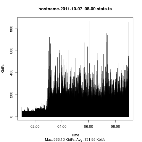
There are sexier graphs out there but from a functional standpoint it does the job.

Combining graphs

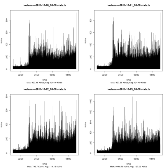
R is fully capabale of creating a collection of graphs from a bunch of files but personally I think it's a lot more involved than simply using ImageMagick's montage command.

montage -geometry <Width>x<Height> <GraphFiles> <OutputGraph>

Yields a similar graph like the one below (intentionally downsampled to fit page)